Publication categories
Publications - Engineering aspects
Using geometrical symmetries for effective detection of stealth targets
06/26/2012
A.V.Kramarenko
And von Neumann gave me an interesting idea: that you don't have to be responsible for the world that you're in. So I have developed a very powerful sense of social irresponsibility as a result of von Neumann's advice.
Richard P. Feynman
"Surely You're Joking, Mr. Feynman!"
"Surely You're Joking, Mr. Feynman!"
However, our business is small. Our business - crow, but there is not even dawn!
Vladimir Bogomolov
“August 44”
“August 44”
Let us suppose that there is an idealized radio locator with the task to detect a target with the RCS approaching very small values. We suppose the noise of the locator receiver unit to be non-changeable non-zero and data accumulation when using multiple location is not permissible. We also think that the size of the target shining point is negligibly small compared to the “pencil” beam spot. The method of detection and selection of the decision making threshold are considered close to the theoretical optimum.
It is clear that in this case the detection efficiency with constant RCS of the target and power radiated by the station will depend only on the S/N ratio (signal-to-noise reflected from the target). There is definitely no way to improve the detection characteristics, as we cannot change the signal-to-noise ratio within the framework of the stated problem.
However, let us suppose that there is a method that makes it possible to increase the target detection efficiency under the specified conditions. Let us also suppose that it does not contradict the basic foundations of the theory, which, in essence, is intended for a limited dimensionality of the space, in which the signal is detected. For this purpose we consider the detection process in the form of geometrical model.
We will suppose that the beam has in the image plane the Gaussian distribution of the power flow density. Then a single spot will look as follows.

Fig.1. Beam power distribution in the image plane
The third dimension of this beam will be distance, and we can legitimately suppose that in the three-dimensional space the distribution of power flow density will be a fuzzy cone, the equipower lines of which coincide with the antenna main lobe.

Fig.2. Power distribution in the beam
The power distribution in time of the signal reflected from the target (if the shiny point is on the cone longitudinal axis) corresponds to the signal at the receiver input, the response from target moment corresponding thereat to the distance from the target to the antenna.
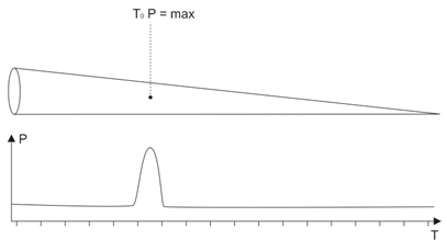
Fig.3. The distance to target unequivocally corresponds to the time of response from target appearance
Thus we have the right to “fill” the cone with the PFD values obtained from location towards the target. That is, roughly speaking, the signal at the receiver input can be converted into a geometric object, where the signal delay time is multiplied by the velocity of its propagation in space and becomes the distance, and the signal instantaneous amplitude is converted into the cone filling intensity. As a result the cone “brightness” is maximum at the distance equal to the distance to target, and at other distances it is proportional to the instantaneous amplitude of noise at the receiver input.
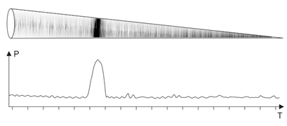
Fig.4. Taking into account the unambiguous correspondence time/distance, we transform the signal at he receiver input into geometrical object filling
In the image plane the result will be a fuzzy spot of the target, quantized by the beams that form the image. In this case we consider not a single beam, but their plurality passed through this image plane. The fact that they have passed through the plane at different times is of no interest for us – we will consider all data to be stored in some virtual memory (for example let there be something like photo emulsion in the image plane exposed by the beams). In this case the signal reflected from the target is stored as well.
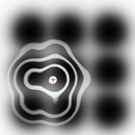
Fig.5. Distribution of equipower lines: the target is in the spot marked by cross. The obtained complex figures are determined by the place of target location in respect to the beam array. Please pay attention that as the power of response from target falls the lines tend to become a circle.
For image planes displaced in respect to the distance to target the received signal distribution will tend to random one specified by air noises, receiver noises and interference (if it is present).
Eventually in 3D space at a posterior analysis of location results the response from target can be considered to be an ellipsoid of revolution.
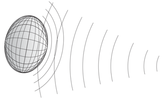
Fig.6. We have right to imagine the response from target in the form of fuzzy ellipsoid
If we consider the shiny dot dimension to be negligibly small, then the crosswise size of this ellipsoid is actually completely determined by the width of the main directional pattern lobe, the degree of compression – by the ratio of the lobe width to the width of response from target (in the time domain), and the brightness – by the shiny spot RCS.
It is clear that the ellipsoid is not in the empty signal space, but in the space filled by actual signals and pseudo signals, the imaginary power of which is determined by the receiver noise level, and the actual power – by air noise and interference. It is also clear that the ellipsoid itself have an additive stochastic component caused by the same noises.
But the locator beams quant the space and, analyzing the location results of some volume of space, we can rightfully represent the input stored data in the form of 3D matrix, and the reflected from target signal – as the brightness values of voxels [1], which fill all analyzed volume. The introduced notion of voxel (in respect to this problem) can be defined as a geometric object, the depth of which corresponds to the locator resolution as to distance, and the dimensions in the image plane – to the resolution caused by beam overlap. Then the response from a shiny point can be represented as shown in Fig. 7.
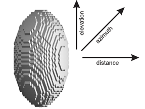
Fig.7. Due to pulse method of locator operation its beams quant the space and we can represent the ellipsoid only as a cloud of voxels, each of them representing a volume of space the minimum value of which is determined by the system resolution limit. That is we can know nothing about power distribution inside the voxel.
Let us note that the region of space filled with signals around the point with the target coordinates is completely symmetrical in respect to this point (if the ellipsoid is degenerated into a sphere) and potentially symmetrical for any ellipsoid at the corresponding proportional compression or stretching of space.
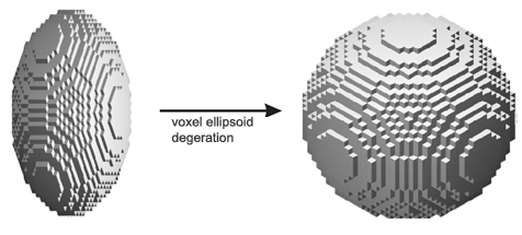
Fig.8. Virtual conversion of asymmetric voxel into symmetric one (if we suppose the resolution as to distance to be better than the resolution as to azimuth/elevation) makes it possible to simplify the calculation of the ellipsoid layer brightness
But for the description of a symmetrical (in respect to the center in all dimensions) object it is sufficient to have the signal power distribution along the Euclidian distance (for the case of sphere – radius). At the same time we have redundant amount of information, resulted from location. And if we ensure 3D convolution of the obtained signal with its 3D prototype determined by the characteristics of the a priori known model of ellipsoid, the S/N ratio (signal/non-correlated with model noise) will be determined not only by the input S/N, but also by the square root of the number of voxels comprising the model (under real conditions the law is somewhat more complicated). In other words, the narrower is the antenna radiation pattern, the better is the resolution as to distance and larger is the model volume, the more efficient accumulation coherent accumulation of non-coherent noise will be ensured. And comparing with the classical method, when the optimal detection is considered to be only the convolution along one dimension (distance), the proposed method will ensure substantial advantage. It is also clear that if we use symmetry only in the target aperture [2], then the limit gain in signal-to-noise ratio is limited by the available dimensionality. And besides, if we use the space around the target (supposing that its region close to the target is free from other targets), its three dimensions make it possible to obtain even more significant advantage.
However, the multi-dimensional convolution (even as FFT) is a rather resource consuming solution. Therefore it is more expedient to use the internal symmetry of forcedly degenerate ellipsoid and “pack” it in one dimension. Let us explain: if the locator resolution as to distance and azimuth/elevation is equal, there are no problems. But usually the resolution as to distance is higher, resulting in the ellipsoid being compressed along the corresponding axis. And the most simple method of fiber symmetry usage will be the recognition of initially compressed voxel as cubic one, that is we will simply “stretch” the space in the vicinity of the target.
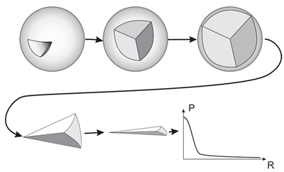
Fig. 9. Summing of voxels belonging to a given layer can be represented as unfolding and compression of a sphere.
In the sense of calculation it will be equivalent to summing all power values for equal radius values. The solution of such problem by the table method will not be connected with any significant computational expenses.
As a result we obtain a chart describing the signal level depending on the voxel distance from the shiny point.
Let us consider the expected form of this chart for the case of actual usage. We suppose at each following tact shifts the beam as to azimuth and/or elevation by the value of antenna radiation pattern one-half power. Then the value of the shiny spot response will have the amplitude 1.414 times smaller at the next tact and 2 times smaller at the second one and so on. That is readings along the ordinate axis will have values 1.0…0.707…0.5…0.354…0.25 and asymptotically approach zero.
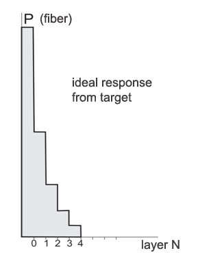
Fig.10. Signal average power in layers related to the maximum possible response from target (layer No.1).
But as the brightness of equally remote from the ellipsoid voxels is equivalent (due to complete symmetry of the figure), the value of signal-to-noise ratio in its layers can be represented by the following table:

It follows from the table that the signal averaging in all voxels of a layer the noise level is reduced by the square root of the number of summed voxels times (we suppose that the noise is not correlated) due to faster drop-down of the noise amplitude in respect to falling down amplitude of the signal in all layers but the zero one, more than threefold of the signal-to-noise ratio is ensured. It is clear that this does not take place in the zero layer, i.e. central voxel. If we sum up the data obtained over all layers, the amplitude signal-to-noise ratio can be increased in this case twofold more. But this will result in the decrease of spatial resolution of the entire system, which is unacceptable (i.e. it will turn out that we use not one beam, but as many, as there are layers in the model, and the resolution as to azimuth/elevation falls down proportionally).
But if we change the scanning principle and/or increase the bean overlapping, the signal-to-noise ratio will additionally increase without the resolution decrease (and this, as it seems, is the most useful “bonus” of the proposed method).
However, here it is necessary to give some explanations. As a paradoxical (at first sight) conclusion follows from the table that the work on target is more effective for the cases when the antenna “looks somewhat aside”, the experimental proof will be quite appropriate.
Let us specify an arbitrary (knowingly small) signal-to-noise ratio at the demodulator output (but before the threshold device).
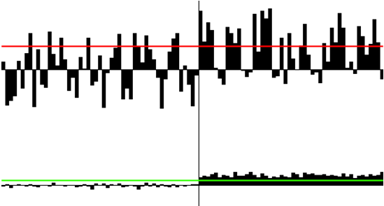
Fig. 11. Upper diagram – signal values when measuring the central voxel, lower one – the sum of signals in voxels of all layers except the central one. Along X-axis – time, along Y-axis – quantized levels of the demodulator output. The left-hand part of the diagrams corresponds to the absence of useful signal at the input, the right hand one – a constant signal has appeared in all voxels. Its level falls down as the distance from the central voxel increases according to the antenna radiation pattern.
Fig.11 illustrates (a specially developed program was used for modeling) the case when the measurement in the central voxel (that is classical radiolocation method) do not permit to select the Bayesian threshold that ensures an acceptable value of errors of the first/second kind. That is, roughly speaking, the signal is not detected at all. At the same time the lower diagram demonstrates timely and error-free signal detection on the background of noises. Naturally, at multiple location and data accumulation one can detect the signal by the usual method as well, but the formulated problem – do not use accumulation – excludes this version.
Surely, the simplest set of coefficients is used in this case, which supposes that the antenna radiation patterns will be as follows:
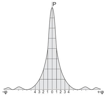
Fig. 12. Antenna radiation pattern that corresponds to the coefficients used in the considered model.
It is clear that the actual radiation pattern will differ and signal-to-noise ratios in the layers will be different. We must take thereat into account that the adaptation of the scanning algorithm taking into account specific features of the antenna radiation pattern can yield a considerably greater gain in the signal level in respect to noises. Even more, if the scanning method has one-half shift of line in even and odd columns, the filling will become hexagonal one, and voxel will be a hexagonal prism. However, consideration of the method optimization questions seems premature yet.
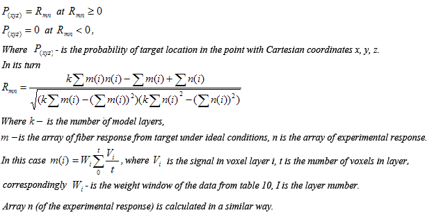
Execution of the described geometric transform will result in the signal describing the correspondence of the accepted model data. In this case the degree of correspondence to the prototype is equivalent to the probability of the target being in the point of space, which coincides with the model center.
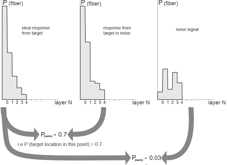
Fig.13. Decision making algorithm when comparing fibered responses from the target. Here P(norm) are the values of Pearson correlation coefficient and at the same time the probability of the target being in the point with the coordinates coinciding with the central voxel coordinates. The response from target is always compared to the reference, i.e. ideal response.
Calculation of the normalized correlation of the obtained sequence with the reference one (which corresponds to the ideal response from target) transforms all data into one output value, which is equivalent to averaging for non-correlated processes.
We must remember that both the signal and the prototype must be multiplied by the data weight window, which is the signal-to-noise ratio for corresponding layers.
Thus, with good approximation we can suppose the noise influence to be reduced by square root from the number of ellipsoid analyzed layer times. In our case it will be not less than twofold amplitude relation. And the summary gain can be estimated as sixfold amplitude one, i.e. by 26 times as to power. For the optimum scanning algorithm and antenna radiation pattern adapted to the proposed method the gain will be even more significant, but, according to the author’s opinion, such work will be a considerable mathematical difficulty. However, it is not excluded that a simple and handsome solution exists.
Sequentially shifting the model (lag from the current location will be the number of tacts equal to one-half of the required number of voxels), we obtain a usual location result, but with a considerably better signal-to-noise ratio, which will ensure the increased target detection distance and larger tolerance of AWGN interference.
And if, instead of Pearson correlator, we use the usual method of calculating the signal convolution with its prototype, the output data will be received in more usual format, which, although requiring normalizing as to output amplitudes, still offers the possibility to estimate energy of response from target. In this case it is necessary to estimate the expected value of spatial resolution of the entire model taking into account the introduction of the fiber model. Let us take into account that in the classical method the resolution as to azimuth/elevation is determined by the width of the radiation pattern main lobe and beam overlapping coefficient, and in the proposed one – by the convolution of ideal fiber response from target with itself.
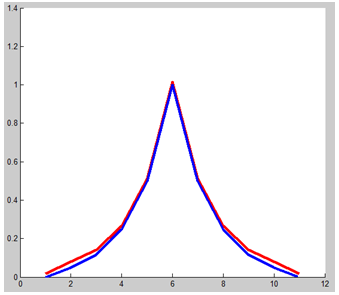
Fig.14. Discrete response from target, stipulated by the antenna radiation pattern (in Fig.12). The red kinked curve is the usual method of RL data processing, the blue one is the convolution of the ideal response from target (Fig. 10), that is the proposed method. We must expect that differences in the obtained target image will be small, and the spatial resolution will not fall down, but even will be somewhat improved.
We must also note that the increase in signal-to-noise ratio is provided in the method being investigated exceptionally by geometry and can be easily subjected to approximate calculation, although, surely, it will be more correct to compare Laplacians of various dimensionalities.
Let us try to confirm experimentally the given figures. For this, we will use a model with previously recorded noise sequence and increase the noise level till the moment when the number of errors of the first and second kind will remain zero in the proposed method. Then, lowering the noise level, we will obtain the zero number of errors for the classical method as well.
Here we must stipulate that such approach to the problem is not completely correct, even more, such hob-a-nob treatment of noise-like signals is bad manners, but, nevertheless, the experiment will make it possible to obtain a rough approximate estimate and avoid at the same time many pages of analytical proof.
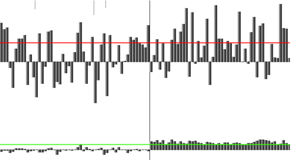
Fig. 15. The noise level is such that only the proposed method (diagram below) ensures zero quantity of errors when detecting the signal (naturally, for the given noise sequence). We must indicate once more that additional processing methods can extract the useful signal from the upper diagram as well, but this will require data accumulation, and in our case the multiple location is not allowed by definition.
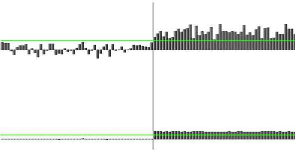
Fig.16. To “bring” the classical method to zero quantity of errors (for the same noise sequence), we had to reduce the noise amplitude fivefold. Naturally, the signal level was not changed.
The obtained coefficient not badly agrees with the previous estimate – the case is that here we separately use the data from the central voxel and summed fiber data. When using the data of all layers, including the zero one, we can hope namely on the sixfold gain in amplitude signal-to-noise ratio.
Let us try, with a program model, to illustrate the obtained result in respect to the target track. Let the target RCS increases from zero to some arbitrary value (so that the signal amplitude linearly grows at the input), at which the track becomes continuous for both methods of RL signal processing (Fig. 17).
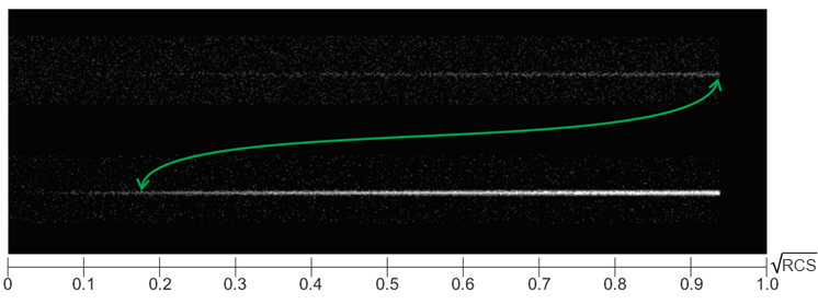
Fig.17. Target tracks with linearly increasing RCS on the background of noises. Above is the usual method of detection, below is the proposed one. The signal before the threshold device. The noise level is normalized, i.e. the images can be compared.
It is obvious that the proposed method makes it possible to obtain without coherent accumulation of signal not less than 25-fold gain in RCS values and, correspondingly, increase in target detection distance in 2.2 times at unchanged transmitter power and receiver sensitivity. This, surely, justifies the attempts to use it in actual practice. However, this very actual practice, being implemented, adores to present problems. For example, for a high-velocity circuit and/or very large distance to target a problem of ellipsoid deformation appears because during the time of required tacts the target will succeed in shifting. Adaptation of the antenna radiation pattern to the proposed method and optimization of coefficients, as well as the selection of the best method of scanning will be a hell of a present. Although a promising one…
So, the algorithm of the device operation (software, the hardware is not changed) will look approximately as follows:
From the receiver demodulator output (but before the threshold detector) the signal is applied to a memory, which fills the memory cells with received values according to the scanning method. In our case 9х9х9 elements are required. Upon filling in of all cells, performed is the weighed summing of signals in voxels, belonging to the layers of corresponding numbers, and a layer brightness table is obtained at the output. These values are applied to a Pearson correlator, the prototype of which is the layer brightness table, experimentally obtained by this locator for a single small-dimension target under the absence of interference. The output value of the normalized correlation is the probability of target detection in the point, corresponding to the ellipsoid center. The cycle is repeated as data are accumulated and analyzed point shifts.
Thus, the probability of the target being in the point with coordinates x, y, z will be determined by the method indicated below.
If it is necessary to obtain the value of the shiny point brightness, we can use a common convolution of the fiber response from target with the reference, and apply the result to a non-linear device that forms the Bayes threshold.
As a conclusion we can say the following:
The proposed method is not a version to improve signal-to-noise ratio, connected with the beam control. That is, the existing methods of aimed analysis of threatened sectors, multiple location of a selected sector, “interference burning through” and so on and so on, always envisage adaptive control over the scanning method. The method of using geometric symmetries does not require changing the scanning algorithm during operation and therefore compliments the indicated classical methods and can be used simultaneously with them. The improvement in signal-to-noise ratio in this case will be multiplied (please, NB!).
The expected gain in signal-to-noise ratio will lead to a multiple equivalent increase of the target RCS, which, most likely, will make in many aspects senseless the «Stealth» technology, as reaching super small RCS already has almost reached the theoretical threshold. And the necessity to lower the RCS several times more has, apart from physical limitations, also economic ones. Although “chillers” about head-on attack on a prepared modern air defense only by stealth aircraft “in pure sky”, that is without coverage by active interference already belong to yellow press kingdom.
As it seems to the author, the method may be useful at head-on long-distance detection of aircraft by each other. The equivalent gain by dozens of times as to power and by two times as to distance at equal RCS of the aircraft unambiguously will enable the one of them, which uses the proposed method, to obtain the decisive advantage in selecting the moment and method of attack. But the questions of tactical application are beyond the competence of the signal processor.
The most significant and principally important, from my point of view, advantage will be the possibility of obtaining (by means of normalized correlation) an RL image in the form of densities of target location probability. Then, processing, as hypothesis, all physically non-contradictive target tracks (we say nothing on computational expenses) and integrating over the track, we can additionally lower the threshold of detection on background of noises by many times.
Category:
- Log in to post comments
PO box 11515, 61001 Kharkov Ukraine,
tel./fax: +38(050)0113940, +38(057)7290409
E-mail: tredex@tredex-company.com
tredex.office@gmail.com